
100-year precipitation intensity in California
We know the atmospheric rivers pummeling California are generating huge amounts of rain. I’ve seen many images and data showing rainfall amounts, but not much information that presents the precipitation amounts in terms of return periods. (Precipitation accounts for both solid and liquid phases of H2O, e.g., snow and rain.) This post examines precipitation in terms of return periods and focuses on the spatial distribution of precipitation on January 9, 2023. Assessing precipitation forecasts in terms of return periods can provide situational awareness and insights into the potential impacts from excessive precipitation.
For context, we start with an example of precipitation observations taken on January 9, by a weather station at Shaver Lake in California (Station: Big Creek PH 1, Site ID: 04-0755, Latitude: 37.2266°, Longitude: -119.2206°). The record shows the station collected almost 8” (~200 mm) of rain over the 24-hour period between 11:56pm on January 8 and 11:56pm on January 9.
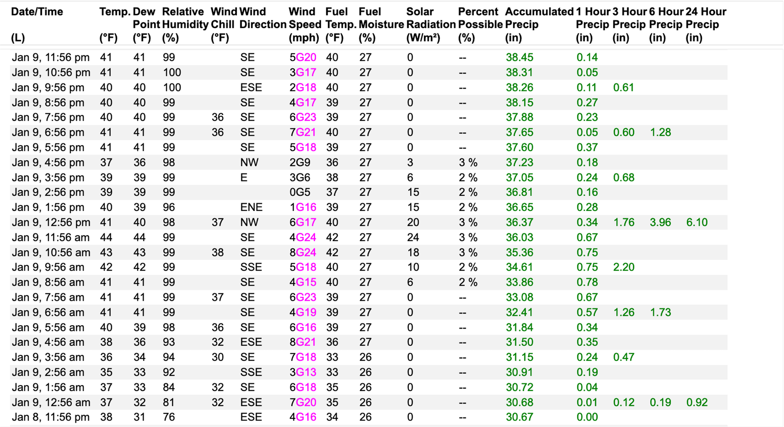
Time series of station data such as that from Shaver Lake can be used to determine precipitation intensity over specified return periods and duration. NOAA provides such estimates at locations where the data are collected and provides maps derived by interpolations among stations.
The figure below shows an example of NOAA’s analysis of precipitation at Shaver Lake. The return period for the 8” of measured precipitation at that point falls between ~15 and ~100-year return period based on the 90% confidence interval. Note that I qualify this by stating “at that point.” Most people care about precipitation in places other than where weather stations are located, and precipitation is incredibly heterogeneous, especially in areas with a lot of topography. What occurs at a point can differ substantially for what occurs a short distance away.

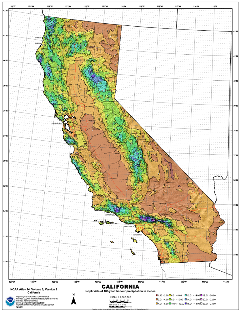
Fortunately, point-specific data from weather stations can be used to generate spatial maps of precipitation return periods. An example of the spatial distribution of 100-year return period precipitation intensity for California is shown in the figure below. The map is provided by NOAA and based on data collected by over 320 stations throughout the state. Note the variability in precipitation in mountainous areas of the state. Information such as this can be used as a reference point to understand the amount of precipitation that might be expected from relatively extreme events across the state. This information can also be compared with precipitation forecasts to get a qualitative sense of the expected impacts from a precipitation event.
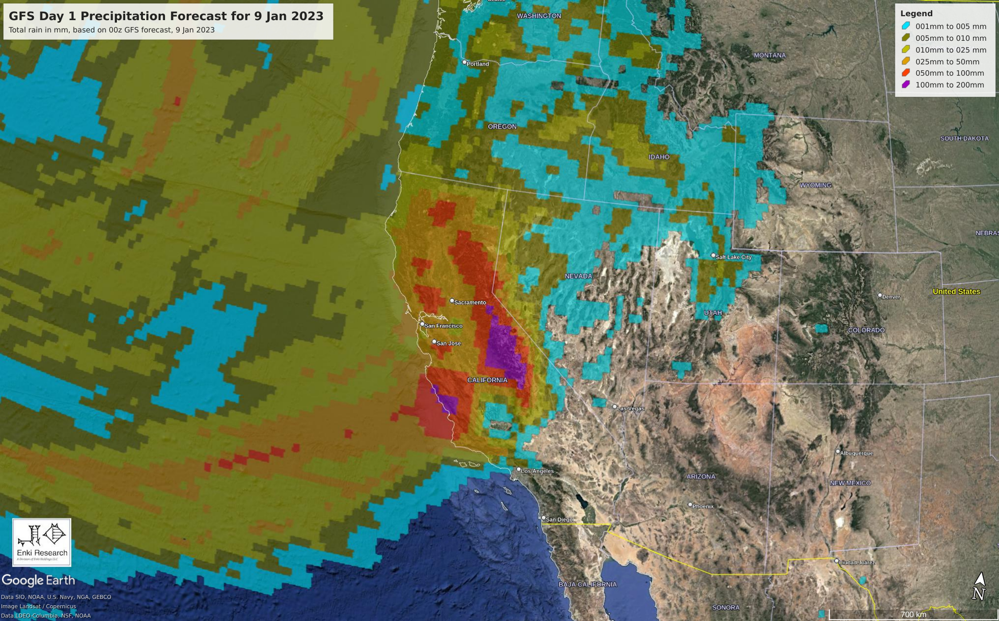
Let’s consider the Global Forecast System (GFS) weather model’s Day 1 Precipitation Forecast for 0:00 GMT (written as 00z) on 9 January 2023 and how it compares with return periods. This forecast is for the same day of precipitation records shown in the first Table. As shown in the figure below, for large areas of the California coast and the Sierra Nevada mountain range, the 24-hour forecast is for more than 100 mm (100 mm ≈ 4 inches) of precipitation. (This figure and the following two are generated by Kinetic Analysis Corporation’s Director of Research, Chuck Watson.) By comparing forecast precipitation with the values shown in the map above, one can see that for some areas, such as the southern Sierra Nevada, the precipitation forecast is significantly less than 100-year return period event. In other areas, such as the coast north of Santa Barbara, the forecast precipitation is equal to or greater than a 100-year event. Notably, recall that these estimates are based on a limited set of point station data distributed unevenly across the state.
Typically, people are interested in precipitation forecasts created a day or more in advance for broad areas that range from neighborhoods to entire river basins. While there are exceptions, this information usually comes from models generated by meteorological agencies. However, unless you are a specialist, you might not know how the forecasts of precipitation compare to a typical amount of rain for an area. You could determine that by comparing the forecast to maps of return period precipitation intensity. But, combining return period intensities with forecasts would be a more convenient solution. Doing so would provide you with a more direct sense of the severity of an event and increase your situational awareness.
Where can one find data on return periods that are appropriate for use precipitation forecasts? Ideally, you’d have a set of reference data that matches the scale of forecast data. As the GFS model provides global forecasts, and many areas of the world have only limited time series of precipitation data, satellite data or reanalysis data prove to be useful for estimating precipitation intensity at different return periods. Examples of time series data that can be used include the NASA GPM/IMERG Level 3 data and reanalysis data such as the Japanese Meteorological Agency’s 60-year reanalysis. Two advantages of satellite and reanalysis data are their global coverage and the fact that they provide spatially averaged values instead of point-specific values. Thus, return periods derived using these data can be used with forecasts generated by global models like GFS.
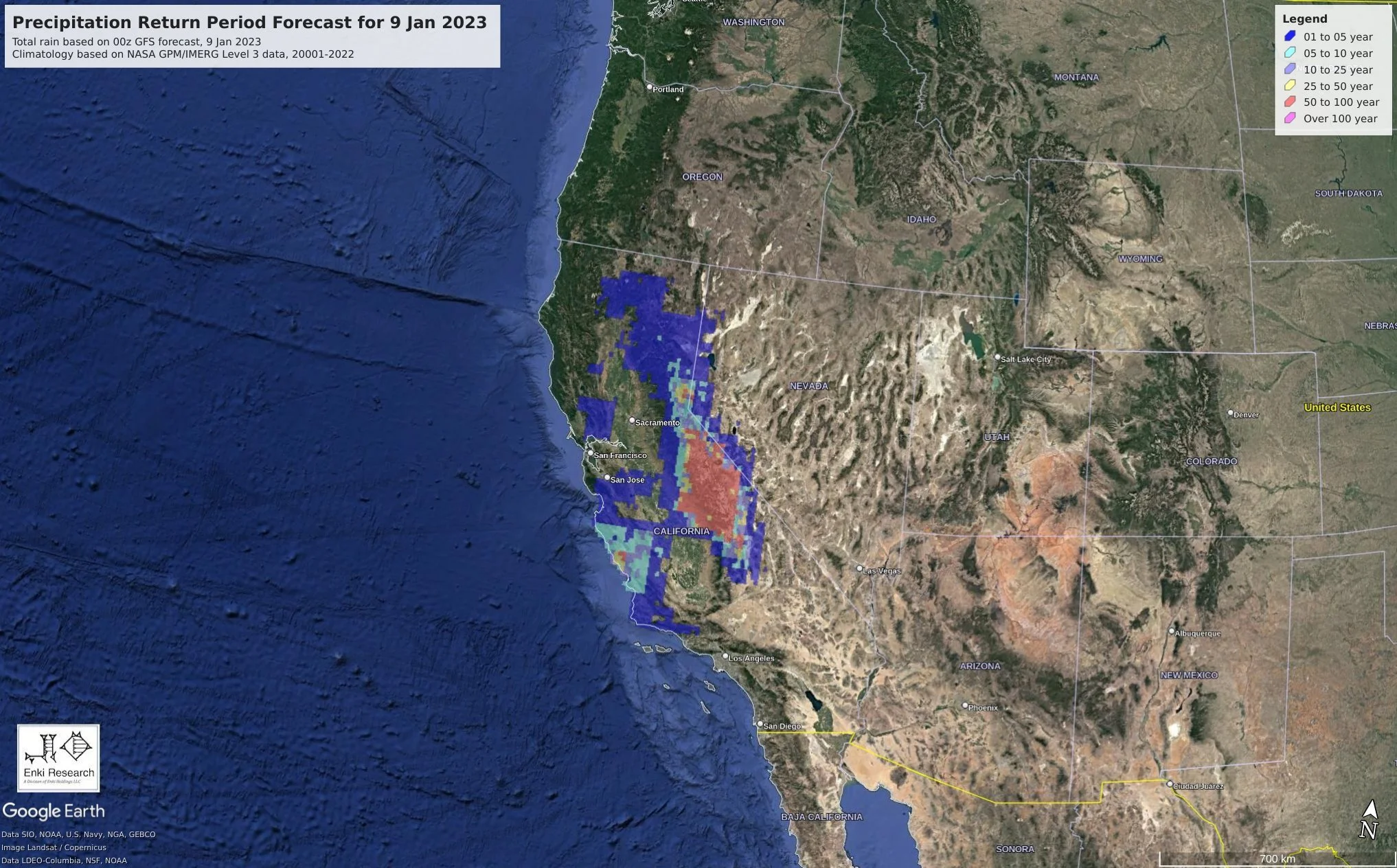
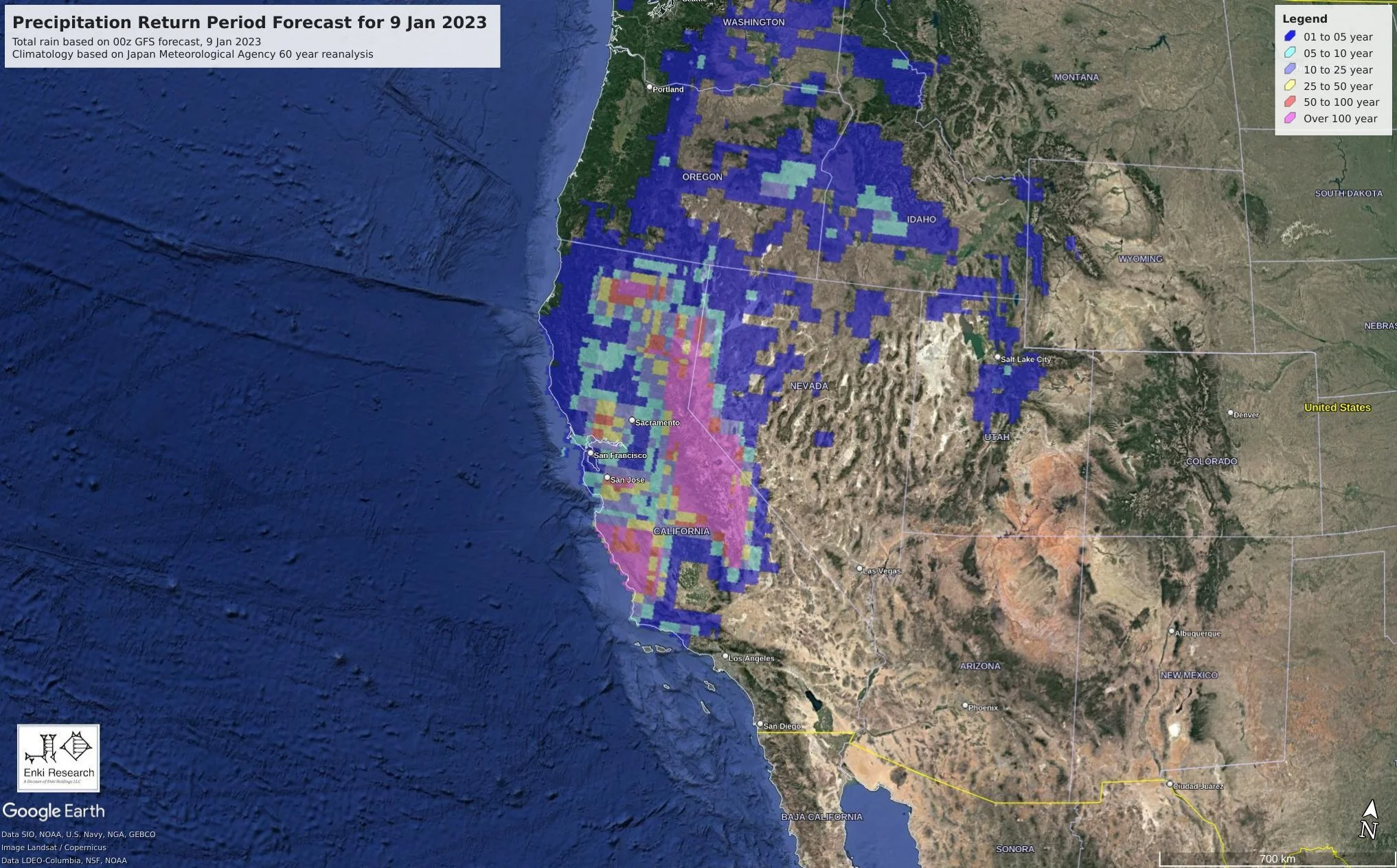
Below we show two images depicting forecasts of precipitation in terms of return periods for a single day, January 9, based on the same GFS forecast shown figure above. The two figures are based on return periods calculated using different time series of precipitation data. The top figure shows precipitation forecasts in terms of return periods based on NASA GPM/IMERG Level 3 data over the 2001-2022 period. The bottom figure shows precipitation forecasts in terms of return periods based on 60 years of Japan Meteorological Agency reanalysis data. The return period intensities are broadly similar. Areas with 100-year return periods span a large area of the Sierra Nevada mountains and foothills and an area north of Santa Barbara.
Given the intensity of the rain relative to historical experience, and the fact that this precipitation would follow multiple days of wet weather, it is not surprising that there are such intense flooding and impacts. These consequences are consistent with the progression of the ongoing atmospheric rivers, which we discuss in more detail in this blog post.
Knowing what to expect is critical to protecting yourself and your businesses. Kinetic Analysis can provide this information on a global basis. If you’re interested, reach out to us at sales@kinanco.com